
Table of Contents
So far we have talked about the uninformed search algorithms which looked through search space for all possible solutions of the problem without having any additional knowledge about search space. But informed search algorithm contains an array of knowledge such as how far we are from the goal, path cost, how to reach to goal node, etc. This knowledge help agents to explore less to the search space and find more efficiently the goal node.
The informed search algorithm is more useful for large search space. Informed search algorithm uses the idea of heuristic, so it is also called Heuristic search.
Heuristics function: Heuristic is a function which is used in Informed Search, and it finds the most promising path. It takes the current state of the agent as its input and produces the estimation of how close agent is from the goal. The heuristic method, however, might not always give the best solution, but it guaranteed to find a good solution in reasonable time. Heuristic function estimates how close a state is to the goal. It is represented by h(n), and it calculates the cost of an optimal path between the pair of states. The value of the heuristic function is always positive.
Admissibility of the heuristic function is given as:
- h(n) <= h*(n)
Here h(n) is heuristic cost, and h*(n) is the estimated cost. Hence heuristic cost should be less than or equal to the estimated cost.
1. Pure Heuristic Search:
Pure heuristic search is the simplest form of heuristic search algorithms. It expands nodes based on their heuristic value h(n). It maintains two lists, OPEN and CLOSED list. In the CLOSED list, it places those nodes which have already expanded and in the OPEN list, it places nodes which have yet not been expanded.
On each iteration, each node n with the lowest heuristic value is expanded and generates all its successors and n is placed to the closed list. The algorithm continues unit a goal state is found.
In the informed search we will discuss two main algorithms which are given below:
- Best First Search Algorithm(Greedy search)
- A* Search Algorithm
2. Best-first Search Algorithm (Greedy Search):
Greedy best-first search algorithm always selects the path which appears best at that moment. It is the combination of depth-first search and breadth-first search algorithms. It uses the heuristic function and search. Best-first search allows us to take the advantages of both algorithms. With the help of best-first search, at each step, we can choose the most promising node. In the best first search algorithm, we expand the node which is closest to the goal node and the closest cost is estimated by heuristic function, i.e.
- f(n)= g(n).
Were, h(n)= estimated cost from node n to the goal.
The greedy best first algorithm is implemented by the priority queue.
2.1. Best first search algorithm:
- Step 1: Place the starting node into the OPEN list.
- Step 2: If the OPEN list is empty, Stop and return failure.
- Step 3: Remove the node n, from the OPEN list which has the lowest value of h(n), and places it in the CLOSED list.
- Step 4: Expand the node n, and generate the successors of node n.
- Step 5: Check each successor of node n, and find whether any node is a goal node or not. If any successor node is goal node, then return success and terminate the search, else proceed to Step 6.
- Step 6: For each successor node, algorithm checks for evaluation function f(n), and then check if the node has been in either OPEN or CLOSED list. If the node has not been in both list, then add it to the OPEN list.
- Step 7: Return to Step 2.
2.2. Advantages:
- Best first search can switch between BFS and DFS by gaining the advantages of both the algorithms.
- This algorithm is more efficient than BFS and DFS algorithms.
2.3. Disadvantages:
- It can behave as an unguided depth-first search in the worst case scenario.
- It can get stuck in a loop as DFS.
- This algorithm is not optimal.
2.4. Example:
Consider the below search problem, and we will traverse it using greedy best-first search. At each iteration, each node is expanded using evaluation function f(n)=h(n) , which is given in the below table.
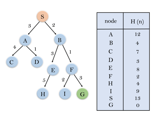
In this search example, we are using two lists which are OPEN and CLOSED Lists. Following are the iteration for traversing the above example.
Expand the nodes of S and put in the CLOSED list
Initialization: Open [A, B], Closed [S]
Iteration 1: Open [A], Closed [S, B]
Iteration 2: Open [E, F, A], Closed [S, B]
: Open [E, A], Closed [S, B, F]
Iteration 3: Open [I, G, E, A], Closed [S, B, F]
: Open [I, E, A], Closed [S, B, F, G]
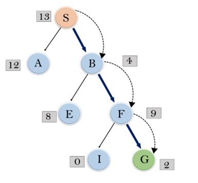
Hence the final solution path will be: S—-> B—–>F—-> G
Time Complexity: The worst case time complexity of Greedy best first search is O(bm).
Space Complexity: The worst case space complexity of Greedy best first search is O(bm). Where, m is the maximum depth of the search space.
Complete: Greedy best-first search is also incomplete, even if the given state space is finite.
Optimal: Greedy best first search algorithm is not optimal.
3. A* Search Algorithm:
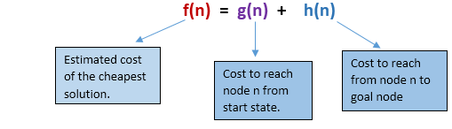
A* search is the most commonly known form of best-first search. It uses heuristic function h(n), and cost to reach the node n from the start state g(n). It has combined features of UCS and greedy best-first search, by which it solve the problem efficiently. A* search algorithm finds the shortest path through the search space using the heuristic function. This search algorithm expands less search tree and provides optimal result faster. A* algorithm is similar to UCS except that it uses g(n)+h(n) instead of g(n).
In A* search algorithm, we use search heuristic as well as the cost to reach the node. Hence we can combine both costs as following, and this sum is called as a fitness number.
At each point in the search space, only those node is expanded which have the lowest value of f(n), and the algorithm terminates when the goal node is found.
3.1. Algorithm of A* search:
Step1: Place the starting node in the OPEN list.
Step 2: Check if the OPEN list is empty or not, if the list is empty then return failure and stops.
Step 3: Select the node from the OPEN list which has the smallest value of evaluation function (g+h), if node n is goal node then return success and stop, otherwise
Step 4: Expand node n and generate all of its successors, and put n into the closed list. For each successor n’, check whether n’ is already in the OPEN or CLOSED list, if not then compute evaluation function for n’ and place into Open list.
Step 5: Else if node n’ is already in OPEN and CLOSED, then it should be attached to the back pointer which reflects the lowest g(n’) value.
Step 6: Return to Step 2.
3.2. Advantages:
- A* search algorithm is the best algorithm than other search algorithms.
- A* search algorithm is optimal and complete.
- This algorithm can solve very complex problems.
3.3. Disadvantages:
- It does not always produce the shortest path as it mostly based on heuristics and approximation.
- A* search algorithm has some complexity issues.
- The main drawback of A* is memory requirement as it keeps all generated nodes in the memory, so it is not practical for various large-scale problems.
3.4. Example:
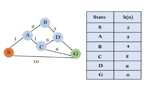
In this example, we will traverse the given graph using the A* algorithm. The heuristic value of all states is given in the below table so we will calculate the f(n) of each state using the formula f(n)= g(n) + h(n), where g(n) is the cost to reach any node from start state.Here we will use OPEN and CLOSED list.
Solution:
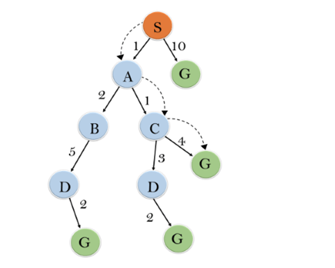
Initialization: {(S, 5)}
Iteration1: {(S–> A, 4), (S–>G, 10)}
Iteration2: {(S–> A–>C, 4), (S–> A–>B, 7), (S–>G, 10)}
Iteration3: {(S–> A–>C—>G, 6), (S–> A–>C—>D, 11), (S–> A–>B, 7), (S–>G, 10)}
Iteration 4 will give the final result, as S—>A—>C—>G it provides the optimal path with cost 6.
Points to remember:
- A* algorithm returns the path which occurred first, and it does not search for all remaining paths.
- The efficiency of A* algorithm depends on the quality of heuristic.
- A* algorithm expands all nodes which satisfy the condition f(n)
Complete: A* algorithm is complete as long as:
- Branching factor is finite.
- Cost at every action is fixed.
Optimal: A* search algorithm is optimal if it follows below two conditions:
- Admissible: the first condition requires for optimality is that h(n) should be an admissible heuristic for A* tree search. An admissible heuristic is optimistic in nature.
- Consistency: Second required condition is consistency for only A* graph-search.
If the heuristic function is admissible, then A* tree search will always find the least cost path.
Time Complexity: The time complexity of A* search algorithm depends on heuristic function, and the number of nodes expanded is exponential to the depth of solution d. So the time complexity is O(b^d), where b is the branching factor.
Space Complexity: The space complexity of A* search algorithm is O(b^d)