
Table of Contents
In this article we list several algorithms for factorizing integers, each of them can be both fast and also slow (some slower than others) depending on their input.
Notice, if the number that you want to factorize is actually a prime number, most of the algorithms, especially Fermat’s factorization algorithm, Pollard’s p-1, Pollard’s rho algorithm will run very slow. So it makes sense to perform a probabilistic (or a fast deterministic) primality test before trying to factorize the number.
1. Trial division
This is the most basic algorithm to find a prime factorization.
We divide by each possible divisor $d$. We can notice, that it is impossible that all prime factors of a composite number $n$ are bigger than $\sqrt{n}$. Therefore, we only need to test the divisors $2 \le d \le \sqrt{n}$, which gives us the prime factorization in $O(\sqrt{n})$.
The smallest divisor has to be a prime number. We remove the factor from the number, and repeat the process. If we cannot find any divisor in the range $[2; \sqrt{n}]$, then the number itself has to be prime.
vector<long long> trial_division1(long long n) {
    vector<long long> factorization;
    for (long long d = 2; d * d <= n; d++) {
        while (n % d == 0) {
            factorization.push_back(d);
            n /= d;
        }
    }
    if (n > 1)
        factorization.push_back(n);
    return factorization;
}
1.1. Wheel factorization
This is an optimization of the trial division. The idea is the following. Once we know that the number is not divisible by 2, we don’t need to check every other even number. This leaves us with only $50\%$ of the numbers to check. After checking 2, we can simply start with 3 and skip every other number.
vector<long long> trial_division2(long long n) {
    vector<long long> factorization;
    while (n % 2 == 0) {
        factorization.push_back(2);
        n /= 2;
    }
    for (long long d = 3; d * d <= n; d += 2) {
        while (n % d == 0) {
            factorization.push_back(d);
            n /= d;
        }
    }
    if (n > 1)
        factorization.push_back(n);
    return factorization;
}
This method can be extended. If the number is not divisible by 3, we can also ignore all other multiples of 3 in the future computations. So we only need to check the numbers $5, 7, 11, 13, 17, 19, 23, \dots$. We can observe a pattern of these remaining numbers. We need to check all numbers with $d \bmod 6 = 1$ and $d \bmod 6 = 5$. So this leaves us with only $33.3\%$ percent of the numbers to check. We can implement this by checking the primes 2 and 3 first, and then start checking with 5 and alternatively skip 1 or 3 numbers.
We can extend this even further. Here is an implementation for the prime number 2, 3 and 5. It’s convenient to use an array to store how much we have to skip.
vector<long long> trial_division3(long long n) {
    vector<long long> factorization;
    for (int d : {2, 3, 5}) {
        while (n % d == 0) {
            factorization.push_back(d);
            n /= d;
        }
    }
    static array<int, 8> increments = {4, 2, 4, 2, 4, 6, 2, 6};
    int i = 0;
    for (long long d = 7; d * d <= n; d += increments[i++]) {
        while (n % d == 0) {
            factorization.push_back(d);
            n /= d;
        }
        if (i == 8)
            i = 0;
    }
    if (n > 1)
        factorization.push_back(n);
    return factorization;
}
If we extend this further with more primes, we can even reach better percentages. However, also the skip lists will get a lot bigger.
1.2. Precomputed primes
Extending the wheel factorization with more and more primes will leave exactly the primes to check. So a good way of checking is just to precompute all prime numbers with the Sieve of Eratosthenes until $\sqrt{n}$ and test them individually.
vector<long long> primes;

vector<long long> trial_division4(long long n) {
    vector<long long> factorization;
    for (long long d : primes) {
        if (d * d > n)
            break;
        while (n % d == 0) {
            factorization.push_back(d);
            n /= d;
        }
    }
    if (n > 1)
        factorization.push_back(n);
    return factorization;
}
2. Fermat’s factorization method
We can write an odd composite number $n = p \cdot q$ as the difference of two squares $n = a^2 – b^2$: $$n = \left(\frac{p + q}{2}\right)^2 – \left(\frac{p – q}{2}\right)^2$$ Fermat’s factorization method tries to exploit the fact, by guessing the first square $a^2$, and check if the remaining part $b^2 = a^2 – n$ is also a square number. If it is, then we have found the factors $a – b$ and $a + b$ of $n$.
int fermat(int n) {
    int a = ceil(sqrt(n));
    int b2 = a*a - n;
    int b = round(sqrt(b2));
    while (b * b != b2) {
        a = a + 1;
        b2 = a*a - n;
        b = round(sqrt(b2));
    }
    return a - b;
}
Notice, this factorization method can be very fast, if the difference between the two factors $p$ and $q$ is small. The algorithm runs in $O(|p – q|)$ time. However since it is very slow, once the factors are far apart, it is rarely used in practice.
However there are still a huge number of optimizations for this approach. E.g. by looking at the squares $a^2$ modulo a fixed small number, you can notice that you don’t have to look at certain values $a$ since they cannot produce a square number $a^2 – n$.
3. Pollard’s $p – 1$ method
It is very likely that at least one factor of a number is $B$-powersmooth for small $B$. $B$-powersmooth means, that every power $d^k$ of a prime $d$ that divides $p-1$ is at most $B$. E.g. the prime factorization of $4817191$ are is $1303 \cdot 3697$. And the factors are $31$-powersmooth and $16$-powersmooth respectably, because $1303 – 1 = 2 \cdot 3 \cdot 7 \cdot 31$ and $3697 – 1 = 2^4 \cdot 3 \cdot 7 \cdot 11$. In 1974 John Pollard invented a method to extracts $B$-powersmooth factors from a composite number.
The idea comes from Fermat’s little theorem. Let a factorization of $n$ be $n = p \cdot q$. It says that if $a$ is coprime to $p$, the following statement holds:
$$a^{p – 1} \equiv 1 \pmod{p}$$
This also means that
$$a^{(p – 1)^k} \equiv a^{k \cdot (p – 1)} \equiv 1 \pmod{p}.$$
So for any $M$ with $p – 1 ~|~ M$ we know that $a^M \equiv 1$. This means that $a^M – 1 = p \cdot r$, and because of that also $p ~|~ \gcd(a^M – 1, n)$.
Therefore, if $p – 1$ for a factor $p$ of $n$ divides $M$, we can extract a factor using Euclid’s algorithm.
It is clear, that the smallest $M$ that is a multiple of every $B$-powersmooth number is $\text{lcm}(1,~2~,3~,4~,~\dots,~B)$. Or alternatively: $$M = \prod_{\text{prime } q \le B} q^{\lfloor \log_q B \rfloor}$$
Notice, if $p-1$ divides $M$ for all prime factors $p$ of $n$, then $\gcd(a^M – 1, n)$ will just be $n$. In this case we don’t receive a factor. Therefore we will try to perform the $\gcd$ multiple time, while we compute $M$.
Some composite numbers don’t have $B$-powersmooth factors for small $B$. E.g. the factors of the composite number $100.000.000.000.000.493 = 763.013 \cdot 131.059.365.961$ are $190.753$-powersmooth and $1092161383$-powersmooth. We would have to choose $B >= 190.753$ to factorize the number.
In the following implementation we start with $B = 10$ and increase $B$ after each each iteration.
long long pollards_p_minus_1(long long n) {
    int B = 10;
    long long g = 1;
    while (B <= 1000000 && g < n) {
        long long a = 2 + rand() %  (n - 3);
        g = gcd(a, n);
        if (g > 1)
            return g;

        // compute a^M
        for (int p : primes) {
            if (p >= B)
                continue;
            long long p_power = 1;
            while (p_power * p <= B)
                p_power *= p;
            a = power(a, p_power, n);

            g = gcd(a - 1, n);
            if (g > 1 && g < n)
                return g;
        }
        B *= 2;
    }
    return 1;
}
Notice, this is a probabilistic algorithm. It can happen that the algorithm doesn’t find a factor.
The complexity is $O(B \log B \log^2 n)$ per iteration.
4. Pollard’s rho algorithm
Another factorization algorithm from John Pollard.
Let the prime factorization from a number be $n = p q$. The algorithm look at a pseudo-random sequence ${x_i} = {x_0,~f(x_0),~f(f(x_0)),~\dots}$ where $f$ is a polynomial function, usually $f(x) = x^2 + c \bmod n$ is chosen with $c = 1$.
Actually we are not very interested in the sequence ${x_i}$, we are more interested in the sequence ${x_i \bmod p}$. Since $f$ is a polynomial function and all the values are in the range $[0;~p)$ this sequence will begin to cycle sooner or later. The birthday paradox actually suggests, that the expected number of elements is $O(\sqrt{p})$ until the repetition starts. If $p$ is smaller than $\sqrt{n}$, the repetition will start very likely in $O(\sqrt[4]{n})$.
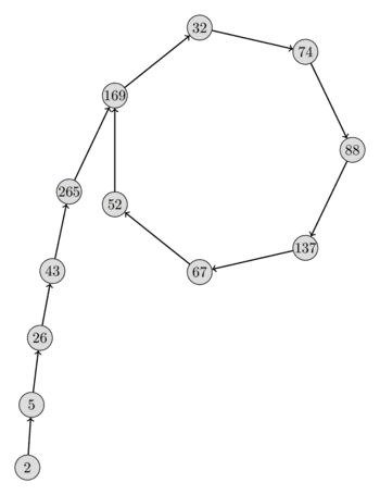
Here is a visualization of such a sequence ${x_i \bmod p}$ with $n = 2206637$, $p = 317$, $x_0 = 2$ and $f(x) = x^2 + 1$. From the form of the sequence you can see very clearly why the algorithm is called Pollard’s $\rho$ algorithm.
There is still one big open question. We don’t know $p$ yet, so how can we argue about the sequence ${x_i \bmod p}$?
It’s actually quite easy. There is a cycle in the sequence $\{x_i \bmod p\}_{i \le j}$ if and only if there are two indices $s, t \le j$ and $t$ with $x_s \equiv x_t \bmod p$. This equation can be rewritten as $x_s – x_t \equiv 0 \bmod p$ which is the same as $p ~|~ \gcd(x_s – x_t, n)$.
Therefore, if we find two indices $s$ and $t$ with $g = \gcd(x_s – x_t, n) > 1$, we have found a cycle and also a factor $g$ of $n$. Notice that it is possible that $g = n$. In this case we haven’t found a proper factor, and we have to repeat the algorithm with different parameter (different starting value $x_0$, different constant $c$ in the polynomial function $f$).
To find the cycle, we can use any common cycle detection algorithm.
4.1. Floyd’s cycle-finding algorithm
This algorithm finds a cycle by using two pointer. These pointers move over the sequence at different speeds. In each iteration the first pointer advances to the next element, but the second pointer advances two elements. It’s not hard to see, that if there exists a cycle, the second pointer will make at least one full cycle and then meet the first pointer during the next few cycle loops. If the cycle length is $\lambda$ and the $\mu$ is the first index at which the cycle starts, then the algorithm will run in $O(\lambda + \mu)$ time.
This algorithm is also known as tortoise and the hare algorithm, based on the tale in which a tortoise (here a slow pointer) and a hare (here a faster pointer) make a race.
It is actually possible to determine the parameter $\lambda$ and $\mu$ using this algorithm (also in $O(\lambda + \mu)$ time and $O(1)$ space), but here is just the simplified version for finding the cycle at all. The algorithm and returns true as soon as it detects a cycle. If the sequence doesn’t have a cycle, then the function will never stop. However this cannot happen during Pollard’s rho algorithm.
function floyd(f, x0):
    tortoise = x0
    hare = f(x0)
    while tortoise != hare:
        tortoise = f(tortoise)
        hare = f(f(hare))
    return true
4.2. Implementation
First here is a implementation using the Floyd’s cycle-finding algorithm. The algorithm runs (usually) in $O(\sqrt[4]{n} \log(n))$ time.
long long mult(long long a, long long b, long long mod) {
    return (__int128)a * b % mod;
}

long long f(long long x, long long c, long long mod) {
    return (mult(x, x, mod) + c) % mod;
}

long long rho(long long n, long long x0=2, long long c=1) {
    long long x = x0;
    long long y = x0;
    long long g = 1;
    while (g == 1) {
        x = f(x, c, n);
        y = f(y, c, n);
        y = f(y, c, n);
        g = gcd(abs(x - y), n);
    }
    return g;
}
The following table shows the values of $x$ and $y$ during the algorithm for $n = 2206637$, $x_0 = 2$ and $c = 1$.
$$ \newcommand\T{\Rule{0pt}{1em}{.3em}} \begin{array}{|l|l|l|l|l|l|} \hline i & x_i \bmod n & x_{2i} \bmod n & x_i \bmod 317 & x_{2i} \bmod 317 & \gcd(x_i – x_{2i}, n) \\ \hline 0 & 2 & 2 & 2 & 2 & – \\ 1 & 5 & 26 & 5 & 26 & 1 \\ 2 & 26 & 458330 & 26 & 265 & 1 \\ 3 & 677 & 1671573 & 43 & 32 & 1 \\ 4 & 458330 & 641379 & 265 & 88 & 1 \\ 5 & 1166412 & 351937 & 169 & 67 & 1 \\ 6 & 1671573 & 1264682 & 32 & 169 & 1 \\ 7 & 2193080 & 2088470 & 74 & 74 & 317 \\ \hline \end{array}$$
The implementation uses a function mult, that multiplies two integers $\le 10^{18}$ without overflow by using a GCC’s type __int128 for 128-bit integer. If GCC is not available, you can using a similar idea as binary exponentiation.
long long mult(long long a, long long b, long long mod) {
    long long result = 0;
    while (b) {
        if (b & 1)
            result = (result + a) % mod;
        a = (a + a) % mod;
        b >>= 1;
    }
    return result;
}
Alternatively you can also implement the Montgomery multiplication.
As already noticed above: if $n$ is composite and the algorithm returns $n$ as factor, you have to repeat the procedure with different parameter $x_0$ and $c$. E.g. the choice $x_0 = c = 1$ will not factor $25 = 5 \cdot 5$. The algorithm will just return $25$. However the choice $x_0 = 1$, $c = 2$ will factor it.
4.3. Brent’s algorithm
Brent uses a similar algorithm as Floyd. It also uses two pointer. But instead of advancing the pointers by one and two respectably, we advance them in powers of two. As soon as $2^i$ is greater than $\lambda$ and $\mu$, we will find the cycle.
function floyd(f, x0):
    tortoise = x0
    hare = f(x0)
    l = 1
    while tortoise != hare:
        tortoise = hare
        repeat l times:
            hare = f(hare)
            if tortoise == hare:
                return true
        l *= 2
    return true
Brent’s algorithm also runs in linear time, but is usually faster than Floyd’s algorithm, since it uses less evaluations of the function $f$.
4.4. Implementation
The straightforward implementation using Brent’s algorithms can be speeded up by noticing, that we can omit the terms $x_l – x_k$ if $k < \frac{3 \cdot l}{2}$. Also, instead of performing the $\gcd$ computation at every step, we multiply the terms and do it every few steps and backtrack if we overshoot.
long long brent(long long n, long long x0=2, long long c=1) {
    long long x = x0;
    long long g = 1;
    long long q = 1;
    long long xs, y;

    int m = 128;
    int l = 1;
    while (g == 1) {
        y = x;
        for (int i = 1; i < l; i++)
            x = f(x, c, n);
        int k = 0;
        while (k < l && g == 1) {
            xs = x;
            for (int i = 0; i < m && i < l - k; i++) {
                x = f(x, c, n);
                q = mult(q, abs(y - x), n);
            }
            g = gcd(q, n);
            k += m;
        }
        l *= 2;
    }
    if (g == n) {
        do {
            xs = f(xs, c, n);
            g = gcd(abs(xs - y), n);
        } while (g == 1);
    }
    return g;
}
The combination of a trial division for small prime numbers together with Brent’s version of Pollard’s rho algorithm will make a very powerful factorization algorithm.